Mechanical application of correct methodologies does not guarantee correct results
Using the weighted average cost of inventory is an acceptable method for financial reporting, which reflects information about past events. However, using the weighted average cost of inventory to choose between alternative options can lead to managerial decisions that destroy company value.
Let’s consider an example from a real business*.
The Production Context
The enterprise produces three main types of products:
- Product 1: Charcoal
- Product 2: Ethyl Acetate (EA)
- Product 3: Urea-Formaldehyde Resins (UFR)
The production of Charcoal is based on an exothermic chemical process, meaning it releases heat. Conversely, the production of EA and UFR uses endothermic chemical processes, meaning they absorb heat.
The heat generated during Charcoal production is transferred in the form of heated steam for the production of EA and UFR, as well as for internal needs (heating). Additionally, steam can be produced by switching on the company’s own natural gas boiler.
The Cost Discrepancy
- Cost of steam obtained during Charcoal production: 14 UAH/Gcal
- Cost of steam obtained using natural gas: 412 UAH/Gcal
Constraints and Cost Structure For Charcoal production, the limiting factor is production capacity (market capacity allows selling significantly more product with a sufficient margin buffer).
In the variable cost structure for UFR production, the cost of steam constitutes:
- Using steam from Charcoal production: 0.1%
- Using steam from the boiler (natural gas): 3.4%
At the current price level, the choice of steam source—from own production or the boiler—is not critical for deciding on the UFR production volume. The limiting factor here is the demand of major buyers.
In variable costs for EA production, the cost of steam constitutes:
- Using steam from Charcoal production: 0.8%
- Using steam from the boiler (natural gas): 17.5%
The Decision Dilemma
Contracts for the sale of EA are concluded monthly before the start of the planned month. There are several dozen potential buyers. The difference in sales prices (calculated on a single delivery basis) is up to 30% or higher.
To produce EA at full capacity, steam from Charcoal production is insufficient, raising the question of the feasibility of turning on the boiler and using natural gas for steam production.
The Management Trap
The company used the Weighted Average Cost method for inventory valuation. Previous management repeatedly tried to analyze this situation, but no clear correlation between EA production volumes and profit was found.
The algorithm used was as follows:
- For preliminary sales planning, orders for EA were selected at prices higher than the variable cost of EA in the previous month.
- Raw material purchases and EA production were planned based on the planned sales volume (taking inventory into account).
- The cost of planned EA production was calculated based on planned raw material purchase prices and other direct costs.
- The obtained planned variable cost was compared with the minimum planned sales prices. Sales volumes were adjusted if necessary. The full cost of planned sales was calculated, and planned profit was determined.
Crucially: The cost of steam used for EA production was calculated using the Weighted Average Cost method.
For Example:
The production cost (variable cost) for the previous month was 600 €/ton with a production volume of 1,800 tons.
Planned sales are presented in the Table 1:
| Quantity, tons | Price, €/ton | Amount, € |
| 50 | 800 | € 40,000 |
| 100 | 780 | € 78,000 |
| 150 | 760 | € 114,000 |
| 250 | 740 | € 185,000 |
| 400 | 680 | € 272,000 |
| 400 | 620 | € 248,000 |
| 450 | 610 | € 274,500 |
| Total: 1,800 | € 1,211,500 |
The Conventional Analysis
Variable production costs for the planned 1,800 tons would be € 1,080,000 (1,800 t × 600 €/t). Consequently, the contribution margin would be € 131,500 (€ 1,211,500 – € 1,080,000).
The Commercial Director assumes that every sale priced above the variable cost increases profit. For calculations, there is only one cost for this type of product, correctly calculated using an acceptable method (Weighted Average Cost). At first glance, the logic seems flawless—the minimum selling price (610 €) is higher than the variable cost (600 €).
A familiar picture, isn’t it?
The Hidden Reality
However, inventory cost is the sum of expenses to obtain a specific type of inventory. In reality, we have two types of steam: steam from Charcoal production and steam from the boiler (natural gas).
The cost of these steam types differs by more than 25 times (!). Consequently, we have two batches of finished goods with different costs:
- “Cheap EA” made with cheap steam (no natural gas).
- “Expensive EA” made with expensive steam (using natural gas).
We can produce a limited quantity of EA using cheap steam, and we can produce an additional quantity using expensive steam.
A New Planning Algorithm: Profit Maximization
Therefore, I changed the planning procedure for EA production and sales to the following algorithm:
- First, we plan the sale of “Cheap EA” (the limited quantity produced without natural gas) for contracts with maximum prices.
- Then, we plan the sale of “Expensive EA” for the remaining contracts with lower prices, only if the selling price exceeds the variable production cost of this specific “Expensive EA.”
- After this, we determine the total cost of sales and planned profit.
Rule #1:
Sell cheap batches of goods under contracts with maximum prices. Then, sell more expensive batches under the remaining contracts, provided the selling price exceeds their specific variable cost.
For example:
The enterprise can produce 1,800 tons of EA per month.
- Steam from Charcoal production (cheap steam) is sufficient to produce 900 tons of EA.
- To produce an additional 900 tons, we must use steam from the natural gas boiler (expensive steam).
Cost Breakdown:
- Variable cost of EA using cheap steam: 550 €/ton.
- Variable cost of EA using expensive steam: 650 €/ton.
According to the new algorithm, the sales plan will look like this (Table 2):
| Quantity, tons | Price, €/ton | Amount, € |
| 50 | 800 | € 40,000 |
| 100 | 780 | € 78,000 |
| 150 | 760 | € 114,000 |
| 250 | 740 | € 185,000 |
| 400 | 680 | € 272,000 |
| 0 | 620 | 0 |
| 0 | 610 | 0 |
| Total: 950 | € 689,000 |
The Financial Result
Variable production costs for the planned 950 tons will be € 527,500 (900t × € 550 + 50t × € 650). Consequently, the contribution margin will be € 161,500.
Under these conditions, producing and selling a smaller quantity of products according to the new algorithm brings the company € 30,000 in additional profit (€ 161,500 – € 131,500).
Why This Works
The variable cost of EA produced using expensive steam exceeds the minimum sales prices under existing contracts. Therefore, producing EA from expensive steam and selling it under such contracts erodes the profit earned from sales at higher prices.
Using my proposed algorithm in the financial model confirmed its correctness and showed a profit increase of up to € 50,000 per month compared to figures planned using the old algorithm. Thus, changing the planning procedure for the production and sale of just one product brought the enterprise about 0.5 million euros per year.
In the very first month of applying this algorithm, the enterprise received an additional profit of over € 40,000 with a lower sales volume compared to the plan under the old procedure.
Visualizing the Situation
Let’s represent this graphically (Fig. 1):
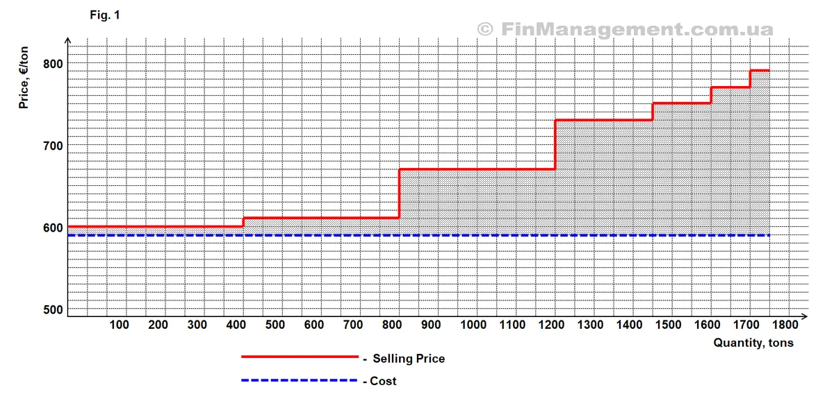
In this graph, the cost is determined using the Weighted Average Cost method. The difference between the sales price and the cost, multiplied by the quantity (i.e., the shaded area between the sales and cost lines), represents the profit.
By separating the cost of products made from differently priced raw materials (steam) in our accounting, we get the following graph (Fig. 2):
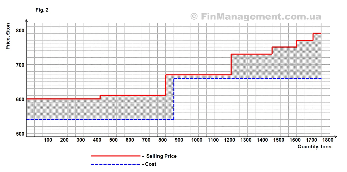
The sales line is above the cost line, meaning all sales are made at a price higher than the cost. Consequently, the more we sell, the more profit we make? From an accounting perspective, everything seems correct.
The Trap Revealed
However, the problem is that increasing sales volume is only possible at prices that are lower than the variable cost of each additionally produced ton of product. Therefore, in this case, increasing sales volume reduces profit.
The sum does not change if we rearrange the addends. Let’s swap the sales at maximum and minimum prices on the graph (according to Rule #1) and we get the following picture (Fig. 3):
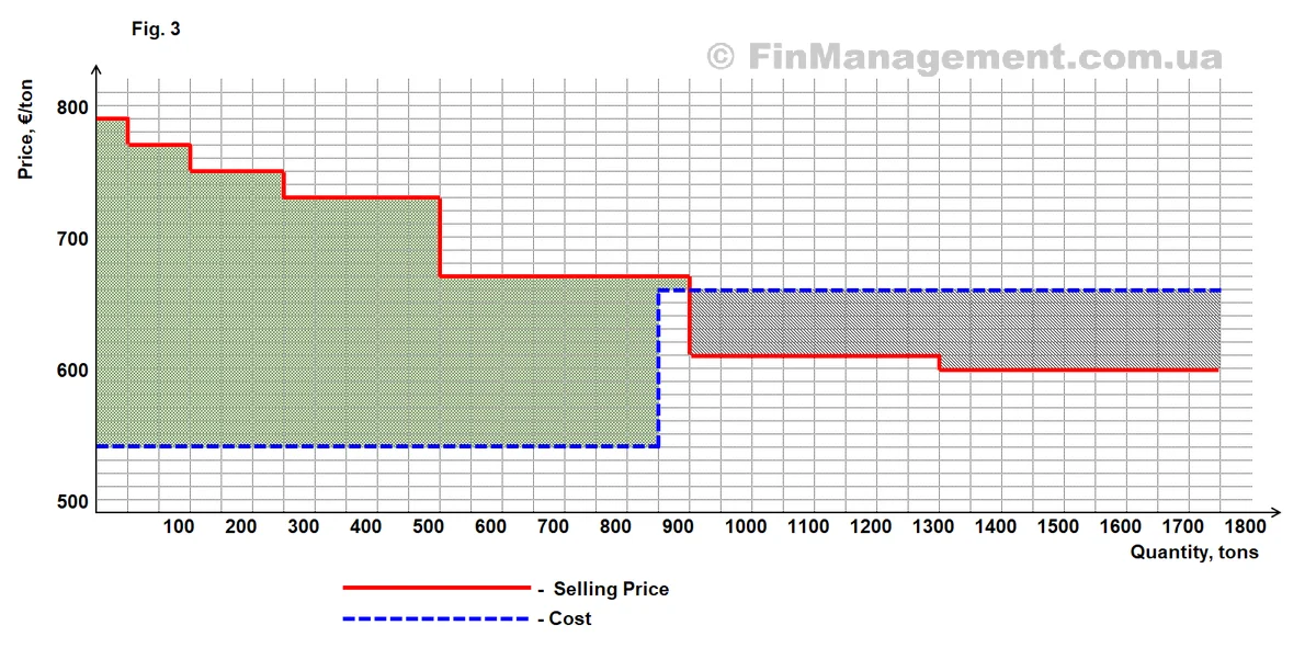
Here, it is clearly visible that all sales at a price below 650 €/ton are loss-making. If we discard them, we achieve maximum profit (the area is shaded and highlighted in color).
Based on the above, we can draw the following conclusion:
Rule #2:
If different batches of raw materials with different prices are used to increase the production and sales volume of a single product type, then to maximize profit, it is necessary to separate the variable production cost in accounting when using cheap and expensive raw materials.
Then, compare the production cost using expensive raw materials with the selling prices. If the variable cost of the product made from expensive raw materials is higher than the minimum selling prices, then such sales reduce profit.
This analysis must be conducted regardless of which inventory valuation method (FIFO or Weighted Average) is used for financial reporting.
It might seem that if we partially allocate the cost of the additional (expensive) steam to the cost of another product (UFR), where its impact on profit is negligible, we could produce and sell more EA at a profit. From an accounting perspective, such a procedure would be correct.
However, by using additional (expensive) steam, we increase the output of only EA. Therefore, for making a decision about the additional volume of EA production, allocating the incremental costs associated with such production to the cost of another product would be incorrect. Such a reallocation of additional costs simply shifts the losses from selling one product (EA) to increasing the cost of another product (UFR).
Consequently, the sale of a larger quantity of product (EA), which looks profitable from an accounting viewpoint, actually reduces the total profit of the enterprise. In other words, if we consider the enterprise as a whole, the incremental costs will be greater than the incremental revenues.
As we can see, the mechanical application of correct (permissible) methodologies does not guarantee correct (optimal) results. An understanding of how value added is formed within the enterprise and a creative approach are essential.
* All numerical values in the example are conditional and show only an approximate order of magnitude.
Published:
- In &.Financier magazine № 1-2, 2010.
- On E-xecutive website — International Community of Managers.
- On Corporate Management website (cfin.ru).
- On Management.com.ua — Internet portal for managers.